Encoding Sunflowers

Back to theory! Today I am writing in a vain attempt to understand this paper by my soon-to-be advisor Anup Rao. I chose it because it seemed interesting and only 6 pages! Little did I know that I was going to be slapped with some of the densest 6 pages I've ever encountered. The goal for this post will be to sprinkle in as much of my intuition as to what is going on as possible, and honestly to try to understand it better myself as I go through with the explanation. There's also a nice talk by Anup, where you can get a lot of intuition but he doesn't have a lot of time to get into the actual details of the encoding. Since that exists but has that shortfall, I'll try and give a bit more details, while still inputting as much intuition as possible.

Finally, I'll mention that the incoming explanation was partly inspired by a recent video from Ryan O'Donnell explaining the famous Switching Lemma from complexity theory. I won't get into what the switching lemma is, but basically a key component of the proof is a clever encoding argument, which O'Donnell describes as leaving clues for a detective. I thought this was both enlightening and cute, so I will attempt something similar, since this proof also involves encodings!

Some Background

The sunflower problem itself is super simple and natural to state, so the background is hopefully quite accessible. Consider a family $\mathcal{F}$ of $\ell$ sets, each of size $k$, where each set is taken from the universe $[n] := \{1, ..., n\}$. Now let's define a sunflower:

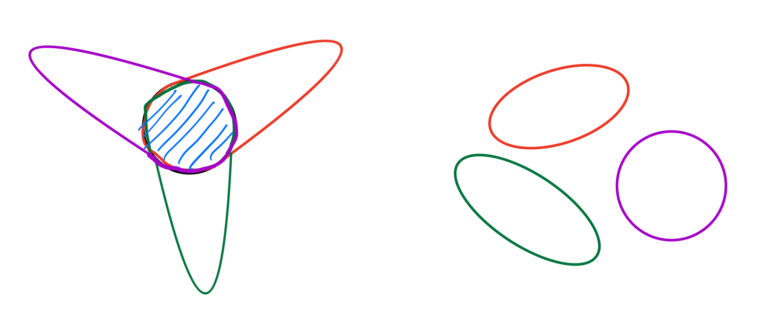
We say that a family of $p$ sets is a $p$-sunflower if all of their intersections are the same.

Sunflower Examples. — Two examples of 3-sunflowers. Note that you can see why they are called sunflowers perhaps from the left example, but totally disjoint sets also count as sunflowers!

The age old question is as follows: how large can we make $\ell$ before we are forced to have a sunflower in our family?

Now I will remark that beyond just being a beautifully simple question to state, the answer to this question has many applications within theoretical computer science. But we won't get into that here, and instead rely on just the beauty of it to motivate us throughout.

Some History: Erdös and Rado showed that if $\ell \geq (p-1)^k\cdot k!$ then there must exist a $p$-sunflower, and moreover, there exists a family with $(p-1)^k$ sets of size $k$ that does not contain a sunflower. They conjectured that this was actually the extremal example, but it wasn't until just a couple of years ago that any progress was made toward closing this gap. Alweiss, Lovett, Wu, and Zhang showed that any family with $\ell \geq (\log k)^k (p \log\log k)^{O(k)}$ sets must have a $p$-sunflower. The paper I am examining today slightly improved and simplified the argument to show that any family with $\ell \geq (\alpha p \log(pk))^k$ sets must have a $p$-sunflower.

Warming Up

So first, the result of Erdös and Rado is simple enough for us to show very quickly, and more importantly offers some intuition as to how subsequent works were able to improve it. So let's take a look! Recall that Erdös and Rado claimed that there must be a $p$-sunflower if $\ell \geq (p-1)^k \cdot k!$.

Case 1: there are $p$ disjoint sets in $\mathcal{F}$. Then this is a sunflower and we are done. Case 2: there are not $p$ disjoint sets in $\mathcal{F}$. Then consider taking the most disjoint sets you possible can, so at most $p-1$, and looking at their union $T$. Note that $|T| \leq (p-1)\cdot k$, and that $T$ intersects every set in $\mathcal{F}$. But then, by an averaging argument, there must be at least one element $i$ that that is in at least $\frac{(p-1)^k\cdot k!}{(p-1)k}$ of the sets. In that case, we can just restrict our view to those sets, take out that element, and apply the inductive hypothesis on this new family of sets of size $k-1$. Oh yeah, this is proof by induction :)

Ok, awesome! Where was the slack in this last proof? Well, it could be that there were more than one element shared by a large portion of the sets in $\mathcal{F}$, which allow for some strong induction argument rather than just regular old induction. The key is to define a concept of how well-spread the family of sets are. If they are well spread, then we should be able to say that there are at least $p$ disjoint sets, and if they are not well-spread, well then we should be able to apply our induction. Let's make this a bit more formal.

We say that a family of sets is $r$-well-spread if for every non-empty set $Z \subset [n]$ the number of elements that contain $Z$ is at most $r^{k-|Z|}$.

Intuitively, we just don't want too many of the sets in our family to contain any single set, as otherwise we would be "concentrated" around this set. In fact, "all" we need to do is show the following lemma:

If a family that has more than $r^k$ sets is $r$-well-spread, then it must contain $p$ disjoint sets.

Why is this all we need to show? Well, if we are not $r$-well-spread, then there exists some $Z$ contained by $r^{k-|Z|}$ sets. We can focus on this new family of sets, take out $Z$ and apply the (strong) inductive hypothesis on this new family of sets to say that there must be a $p$ sunflower. Otherwise, by the lemma, there are $p$ disjoint sets, which is a sunflower.

A High-Level Encoding Schema

What we would like to do, and ultimately will do, is the following. Consider randomly partitioning the universe $n$ into $p$ buckets with $n/p$ elements each. What we like to show is that the probability that a single bucket completely contains one of the sets from our family is greater than $1-1/p$. Then, by a union bound and Markov's inequality, we could show that with positive probability, every bucket compeltely contains one of the sets of our family, immediately showing $p$ disjoint sets, and proving the lemma above.

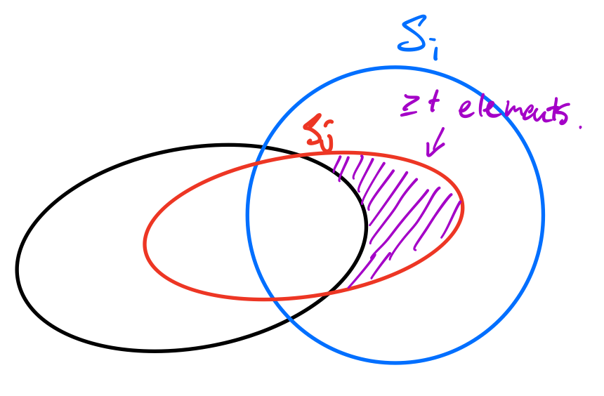
Now, that's a bit difficult, so consider just trying to bound $\Pr[|W \setminus S_i|< t]$ for some $S_i \in \mathcal{F}$ and a random $W$. We can do this by an encoding argument! Specifically, we will encode all of the pairs $(W, S_i)$ where $|W \setminus S_i| \geq t$; i.e. $W$ is not doing a very good job of containing $S_i$. Now, we are going to leave clues for a detective to recover our pair $(W, S_i)$, albeit in a somewhat odd way. This odd way is an attempt to take advantage of our assumption that our family is $r$-well-spread. Here are the clues we leave:

Encode $W \cup S_i$. Naively, this could be any set so there are $2^n$ possibilities here.
Encode $S_j \cap S_i$ for the $S_j \subseteq W\cup S_i$ that minimizes $W \setminus S_j$.

Note that $S_j$ is determined by $W$ and $S_i$.

Now this is just some subset of $S_i$, so there are (again naively) $2^k$ possibilities here.
Encode $S_i$ itself. This is where things get a bit more interesting. Here we can use the assumption that our family is $r$-well-spread to say that there are actually only $r^{k-t}$ possibilities for $S_i$, since $S_j \subseteq S_i$.
Encode $W \cap S_i$. There are at most $2^k$ possibilities here, since this is just some subset of $S_i$ (which we now know from the previous clue).

Now, with these clues, any detective who's any good at their job is able to recover $(W, S_i)$ since they now know both $S_i$ and $W \cap S_i$ and $W \cup S_i$. What was the point with all this? The point is as follows: \[ \begin{align*} \text{# Bad }(W_, S_i) &\leq \text{ # Bad } W \cdot r^k \\ &\leq 2^n \cdot 2^k \cdot 2^k \cdot r^{k-t} \\ &\implies \text{ # Bad } W \leq 2^n \cdot \frac{2^{2k}}{r^t}. \end{align*} \] Where the second inequality comes from our encoding argument. What this tells us is that the fraction of bad $W$ is upper bounded by $\frac{2^{2k}}{r^t}$, so for example if $r$ is some large constant, and $t$ is like $k/100$ or something, then only with exponentially small probability in $k$ do we not pick a good $W$, which in this case is a $W$ that contains 99% of one of the $S_j$.

In some sense, as Rao points out in his talk, this can be thought of as an anti-concentration bound, since we have strong concentration bounds that say that most of the the time $W$ will contain half of any $S_i$, but the above shows, using the well-spread assumption, that it's also extremely likely to contain almost entirely of one of the $S_i$'s. Interesting!

Rao's Encoding

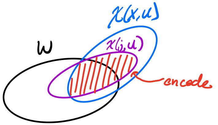
We start with a definition, which hopefully makes sense in light of the previous example. We saw that for a given $S \in \mathcal{F}$, it may not mostly contained in $W$, but somehow there is another $S_j$, which is related to $S$ (being contained in $W \cup S$), which is mostly contained in $W$.

We define $\chi(x, W)$ to be $S_j \setminus W$, where $S_j \subseteq S_x \cup W$ is chosen to minimize $S_j \setminus W$.

Observations:

We are again relating each $S$ (wrt $W$) to some otherset in the family, likely in hopes of using our only assumption, that the family is well-spread.
We don't have to worry about there not being any $S_j \subseteq S \cup W$, since $S$ works and is in the family.
If there is some $S_j$ such that $S_j \subseteq W$, then we immediately have that $|\chi(x,W)| = 0$ for all $W$.

Let $r = \alpha p \log(pk)$ and assume the family is $r$-well-spread. Assume $W$ a uniformly random subset of $[n]$ of size at least $\frac{n}{2p}$ independent of $X$, then we have that $$\mathbb{E}_{X, W}[|\chi(X, W)|] < 1/p.$$ In particular, this implies that $\Pr[\exists j, S_j \subseteq W] >1- 1/p$.

It's easy to see that this lemma is all we need to show. Why? Because we can just take a random partition, and then we have that $$\mathbb{E}[|\chi(X, W_1)| + ... + |\chi(X, W_p)|] < \epsilon p < 1,$$ which implies there must exist some partition that "separates out" $p$ disjoint sets.

Ok, let me state the more technical version of the above lemma, now that we know why we need it.

Let $0 < \gamma, \epsilon< 1/2 $ . Then there exists some $\beta >1$ where if $r = r(k, \epsilon, \gamma) = \beta \cdot (1/\gamma)\log(k/\epsilon)$ and $S_1,...,S_\ell \subseteq [n]$ is an $r$-well-spread sequence of at least $r^k$ sets of size $k$, $X \in [\ell]$ u.a.r., $W \subseteq [n]$ is a uniformly random subset of size at least $\gamma n$ (independent of $X$), then we have that $$\mathbb{E}[|\chi(X,W)|]< \epsilon,$$ which implies $$\Pr_W[\exists y, S_y \subseteq W] > 1-\epsilon.$$

The remainder of the post will be an attempt to convey the ideas in the proof of the above lemma. Rao shows that there exists some constant $\kappa> 1$ such that for each integer $0< m\leq r\gamma/\kappa $, if $W$ is a uniformly random subset of size at least $\kappa m n/r$, then $\mathbb{E}[|\chi(X, W|] \leq k(2/3)^{m}$. Now, note that when $m$ achieves its maximal value of $r\gamma/\kappa$, we get that $\mathbb{E}[|\chi(X, W)|] \leq k\cdot (2/3)^{\alpha \log(k/\epsilon)/\kappa} < \epsilon$ for $\alpha$ chosen to large enough.

Yuck, already too many variables. The point is, we are going to prove this by induction. So what we are going to do is assume that it works for $m-1$, and try to prove it for $m$ (ok, I just said what induction is). How are we going to do that?? Well, we are going to split the $W$ we have, which is of size $\kappa mn/r$ into two disjoint sets, $U$ of size $ u =\kappa (m-1)n/r$ and $V$ of size $v = \kappa n/r$. Then, "all" we have to do is show that for any fixed $U$, we have $$\mathbb{E}_{V,X}[|\chi(X, W)|] \leq2/3 \mathbb{E}_X[|\chi(X, U)|].$$ Ha, easy enough. Of course, without the $2/3$, the above is trivially true.

Let's get a trivial case out of the way. Suppose that $\chi(x, U)$ is empty for some $x$. Recall that $\chi(x, U) = \min_y S_y/U$, where $S_y \subseteq S_x \cup U$. This implies that there exists some $y$ such that $S_y \subseteq U$, which immediately implies that $S_y \subseteq W$, which implies that $$\mathbb{E}[|\chi(X, W)|] = \mathbb{E}[|\chi(X, U)|] = 0,$$ so the bound we are trying to prove would be trivial. So let's suppose that this is not the case, which means that for all $x$, $|\chi(X, U)| \geq 1$.

Encoding $(V, X)$

I promised a detective, now I will deliver. What we are going to do is encode $(V, X)$, meaning we are going to leave clues such that any (mathematically well-versed) detective can recover the pair $(V,X)$. We assume the detective already knows $U$. First of all, how many possible pairs are there? Well, at least $r^k \binom{n-u}{v}$. In fact, exactly that many, and moreover, $X$ and $V$ are uniformly distributed over all the possibilities. By Shannon's arguments, and via Huffman encoding, this means we can encode $(X, V)$ trivially with $log \left ( r^k \binom{n-u}{v} \right )$ bits. But this by itself is not useful to use, and does nothing to relate $\mathbb{E}[|\chi(X, W)|]$ with $\mathbb{E}[|\chi(X, U)|]$, Remarkably, what Rao was able to show is that we can encode $(X, V)$ for our detective using $$log \left ( r^k \binom{n-u}{v} \right ) + a\cdot \mathbb{E}[|\chi(X, U)|] - b \cdot \mathbb{E}[|\chi(X, W)|],$$ which by Shannon's theorem is at least $log \left ( r^k \binom{n-u}{v} \right )$. Crucially, we have that $a/b \leq 2/3$, and this immediately implies the result!

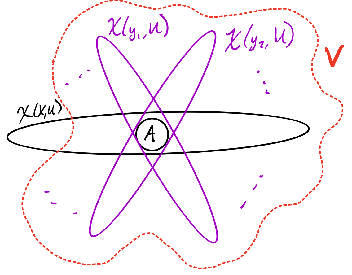
We proceed to encode $(X,V)$ in two different ways, depending on the situation.
Rough case 1: Given some $A \subseteq \chi(X,U)$, there are never too many $y$'s such that $A \subseteq \chi(y,U) \subseteq \chi(X,U) \cup V$. We can utilize this to cleverly encode $X$ with fewer bits than we otherwise might expect, after which the detective knows $\chi(X, U)$, and we just need a bit more information to determine $V$.
Rough case 2: case 1 is not true, so for some $A$ there are lots of possible $y$'s such that $A \subseteq \chi(y,U) \subseteq \chi(X,U) \cup V$. Rao shows that this implies that the number of possible $V$ has now gone down significantly, so we can in this case more cleverly encode $V$ after trivially encoding $X$.

So, we start by defining $$\tau(A, X,V) = \{ y \in [\ell]: A \subseteq \chi(y, U) \subseteq V \cup \chi(X, U) \text{ and } |\chi(y, U)| = |\chi(X, U)|\},$$ and $$\phi(X, V) = r^k (\rho v/n)^{|\chi(X,U)|}\cdot (vr/n)^{-|\chi(X,W)|}.$$ yuck. The point is, that with the above, case 1 is just when $\tau(A, X,V) < \phi(X, V)$ for all $A \subseteq \chi(X, U)$ of size $|\chi(X,W)|$, and case two is, well, when that's not the case. Hopefully it's a bit easier to parse after seeing the rough idea above. Now we are ready to give our detective some clues!

Encoding Case 1

The first bit of this encoding will be zero, to let our detective know that we are in case 1.

Clue 1: encode $|\chi(X,U)|$. Using a trivial encoding, this takes $|\chi(X,U)|$ bits.
Clue 2: encode $W \cup \chi(X,U)$. A simple combinatorial argument upper bounds the length of this encoding.
Clue 3: Let $j$ be such that $\chi(j,U)\subseteq\chi(X,U) \cup W$ and $|\chi(j,U)|$ is minimized. A simple observation is that $j$ could be $X$, so $|\chi(j,U)| \leq |\chi(X,U)|$. We encode $\chi(j,U) \cap \chi(X,U) =: T$. Trivially this can be encoded with $|\chi(X,U)|$ bits.

Visualization of what we are encoding in this step.
Clue 4: First, I claim that $|T| \geq |\chi(X,W)|$. I shan't prove this, so it'll either be an exercise or you can check the original paper if you're curious. The point is, let $A$ be the lexicographically first subset of $T$ of size $|\chi(X,W)|$. The detective will have already used their expert detective skills and knows what $A$ is! Furthermore, by our case 1 assumption, the number of possible $j$ that could've led to producing this $A$ is limited, so we can encode $X$ with only $\log \phi(X,V)$ bits! Brilliant, so we do that.
Clue 5: Now that $X$ is known to the detective, they can infer $\chi(X,U)$. We can then encode $W \cap \chi(X,U)$, and together with $W \cup \chi(X,U)$ the detective can easily figure out $V$.

That's it! I omitted some of the details and algebra, but if you're curious you can check out the original paper. On to case two!

Encoding Case 2

As before, we let the detective know we are in case two by making the first bit 1. Now, we are in case 2, which roughly means that there is some $A$ of size $|\chi(X,W)|$ such that $V$ contains a LOT of other $\chi(y,U)$'s (each of which also contains $A$). This is visualized in the below picture.

What's happening in case 2 — What must happen if we are in case 2.

At a high level, this will limit how many possibilities for $V$ we have.

Clue 1: encode $X$ itself, using $\log r^k$ bits.
Clue 2: $\chi(X,U)$ is now know by the detective, so we can encode the promised $A$ (such that $\tau(A, X, V)$ is very large), which takes at most $|\chi(X, U)|$ bits.
Clue 3: Note that now the detective, being very clever as always, knows $\phi(X,V)$, since $|A| = |\chi(X,W)|$. We proceed to prove that the number of candidates for $V$ is now at most $$\binom{n-u}{v} \cdot (6/\rho)^{|\chi(X,U)|}.$$ Note that for large $\rho$, this is significantly smaller than the trivial bound of $\binom{n-u}{v}$. For your and my sake, I am not going to repeat the proof, but it is not too bad if you want to look! A nice probabilistic argument. This means we can encode $V$ with significantly fewer bits than before.

Rao shows how to put everything together to get the desired bound, but my goal was just to convey the high level idea.

The coolest part by far to me was this notion of using Shannon's information theoretic bounds in this really unique way. Rather than encode the quantity of interest in a normal/canonical way, we do it in a rather weird way in order to get a relationship on the quantities we are interested in. I wonder if this sort of idea works in other settings!

The last thing I will mention is that a super simple modification to the above proof idea was able to give an optimal upper bound of $r = \alpha p \log(k)$ for some constant $\alpha$. Namely, the idea is simple to partition into $2p$ buckets instead of $p$ buckets, and show that with probability $>0$ at least half completely contain a set in the family. Surprisingly, this gets rid of the $\log(p)$ factor! See here for the details, although that's pretty much the entire idea.

← Previous Post Next Post →