Before I begin, James Lee typed up some wonderful notes on parallel repetition, in particular strong parallel repetition, and its connection to the unique games conjecture via max-cut. The latter parts of these notes (and in particular lecture 2) dive into the connections between the odd-cycle game and foams. What are foams? Foams are just tilings of \( \mathbb{R}^d \) by \( \mathbb{Z}^d \) by tiles of unit volume. For an (in fact, optimal) example in \( \mathbb{R}^2 \), see the background image at the top of this post.
I hope to understand this connection with foams a bit better in the future (it's really quite beautiful and clever), but James Lee's notes are already quite nice on this subject, so in this post I am going to avoid beating the dead horse and instead talk about Ran Raz's counterexample to strong parallel repetition. But first, what is strong parallel repetition? What is parallel repetition? There's a lot of background to discuss here, and I will discuss it briefly, but if anything is unclear I refer you to the rest of the internet for sufficient background in order to not make this post ridiculously long.
Some Background
So first, we are going to concern ourselves with 2 prover 1 round games. In this setting, two provers (or players) \(P_1\) and \(P_2\), lets call them Alice and Bob, are trying to convince a verifier \(V\) of something. The verifier samples some \(x \in X\) and gives it to Alice, and also samples some \(y \in Y\) and gives it to Bob. Alice and Bob then, without communicating, must send back \(a\in A\) and \(b \in B\), respectively. \(X\) and \(Y\) are the input alphabets (over which there is some distribution \(\mu\) that the verifier and the provers both know) for Alice and Bob, and \(A\) and \(B\) are the outputs of Alice and Bob. The last thing we need to define the game is the verifier's predicate, which we abuse notation and denote as \(V(x,y,a,b)\). It outputs 1 if the verifier accepts Alice and Bob's answers, and 0 otherwise. Then, the value of the game \(\mathcal{G}\) is $$\mathsf{val}(\mathcal{G}) = \max_{f_A, f_B}\Pr[V(x,y,f_A(x), f_B(y)) = 1],$$ where \(f_A\) and \(f_B\) are Alice and Bob's "strategies". Note that in order for the game to be interesting at all, whatever Aice and Bob are trying to convince the verifier of should not (always) be true. Otherwise, the value of the game is 1, and there is not much to analyze here. I will also note that Alice and Bob are allowed to have shared randomness, but this does not help them. This is because any randomized strategy is just a distribution over deterministic strategies, so they can just pick the best of the deterministic strategies within their distribution.
Now that we have established what a (2 player 1 round) game is, we are ready to introduce the notion of parallel repetition. Suppose we have some game \(\mathcal{G}\) with \(\mathsf{val}(\mathcal{G}) = 1-\epsilon\). For any repetition of \(\mathcal{G}\), we say Alice and Bob "win" iff they win every single repetition. Clearly, if we repeat this game in series \(n\) times then the value of this repeated game will decay exponentially. The central question that we are concerned with here, however, is what happens when we repeat this game in parallel? Repeating the game in parallel means that instead of the verifier sending only one \(x\in X\) and one \(y \in Y\) to Alice and Bob respectively, instead the verifier sends \(x_1,...,x_n \in X\) and \(y_1, ... ,y_n \in Y\) and gets back from Alice and Bob \(a_1,...,a_n\) and \(b_1,...,b_n\), respectively. Let's denote this parallel repeated game as \(\mathcal{G^n}\). Then the value of this parallel repeated game is just the probability that Alice and Bob satisify every predicate, i.e. \(V(x_i, y_i, a_i, b_i) = 1 \,\, \forall i = 1,...,n\).
What is the value of such a parallel repeated game? One might hope or even assume (as some did back when this problem first began gaining attention), that \(\mathsf{val}(\mathcal{G}^n) = (1-\epsilon)^n\); i.e. that the value of the repeated game decays exactly exponentially.
This turns out to be false, which was first shown by Fortnow, and later an even simpler example was described by Feige. The example is instructive, and goes as follows. Consider a game $\widetilde{\mathcal{G}}$ where Alice gets $x \in \{0,1\}$ and Bob gets $y \in \{0,1\}$, and the output alphabets are $A = B = \{1, 2\} \times \{0,1\}$. The verifier's predicate is that both Alice and Bob return either $(1,x)$ or $(2,y)$. It shouldn't be too hard to convince yourself that the value of this game is $1/2$; the best Alice and Bob can do is decide on whether to reply with $1$ or $2$, and then at least one of them has to guess (and with probability $1/2$ they will be right). What happens if we repeat this game in parallel? Here, Alice receives $(x_0, x_1)$ and Bob receives $(y_0, y_1)$. Here is a clever strategy: Alice can return to the verifier $[(1,x_0), (2, x_0)]$ and Bob can return $[(1,y_1), (2, y_1)]$. If $x_0 = y_1$, then Alice and Bob win the parallel repeated game, and this happens with probability $1/2$! Clearly, since the value of the single game is $1/2$, this is also a lower bound for the value of the repeated game, so it turns out the $\mathsf{val}(\widetilde{\mathcal{G}}^2) = 1/2$ for Feige's game.
(Strong) Parallel Repetition
So what do we know about parallel repetition? Clearly, the above example tells us we cannot have "pure" exponential decay in the value of the game if we repeat in parallel. Does the value even have to go to zero as the number of parallel repetitions goes to infinity? Can we have close to exponential decay? Thankfully, for two player one round games, the answer to both of the questions is essentially less (for more than two players, we know that the value goes to zero very slowly, but we don't know very much beyond that). In particular, in the 1990's Verbitsky showed that the answer to the first question is yes using a deep result in Ramsey theory (although, conditioned on knowing that result, the proof is actually quite cute). However, the decay was super slow (shown to be on the order of the inverse Ackermann function, Google it, it's crazy). Shortly thereafter, Ran Raz proved his famous parallel repetition theorem, which showed that for some 2P1R game $\mathcal{G}$, if $\mathsf{val}(\mathcal{G}) = 1-\epsilon$, then we have that $$\mathsf{val}(\mathcal{G}^n) \leq (1-O(\epsilon^c))^{\Omega(n/\log(|A||B|))}. $$ In Raz's original proof (which is, some might argue, a bit less "cute" than Verbitsky's, albeit with the benefit of actually achieving exponential decay), $c=32$, but Holenstein in ~2006 was able to significantly simplify and improve Raz's result to achieve $c=3$ for general 2P1R games. Not long after, for the specific case of projection 2P1R games, Anup Rao showed that if $\mathsf{val}(\mathcal{G}) = 1-\epsilon$, then we have that $$\mathsf{val}(\mathcal{G}^n) \leq (1-O(\epsilon^2))^{\Omega(n)}. $$ Note in particular there is no longer dependence on Alice and Bob's output sizes, and the improved exponent. Strong parallel repetition asks what is the smallest exponent we can achieve, for general 2P1R games or even the specific case of projection games? Rao showed than $c\leq 2$. Is it possible that $c < 2$?
If I had the energy and/or the expertise, now would be a good time to go on a diatribe about why we actually care about optimizing this exponent so much, or indeed why we care about parallel repetition at all. It's an interesting mathematical question! Beyond that, its actually very important in the context of using PCP's to prove hardness of approximation results. At an even finer level of detail, in James Lee's notes linked above he describes how if indeed $c< 2$, even for projection games, this could possibly lead towards a proof of the unique games conjecture. Specifically, if one could show a strong hardness of approximation result for Max-Cut (without assuming UGC), and $c< 2$ (i.e. we had some form of "strong" parallel repetition), then this would imply the unique games conjecture! Again, I will avoid beating the dead horse here since this is already discussed more nicely than I probably would be able to in James Lee's blog. Just trying to give some semblance of motivation here.
Raz's Counterexample
Ok, now that I've gotten your hopes up about just a couple of the cool reasons people would like to see a strong parallel repetition theorem, now I am ready to disappoint. Well, I am always ready to disappoint, but this time I've specifically prepared for the disappointing I am about to do. Let's get into it!
First, I need to introduce the notion of an odd-cycle game. The idea is very simple: Alice and Bob have a cycle on $m=2k+1$ vertices, let's call this graph $C_m$, and are trying to convince the verifier that this graph is 2-colorable. Clearly, it is not (and if it were, then this would not be a very interesting game because Alice and Bob would always be able to convince the verifier). To see this, consider the below picture, where it is clear that at least two neighboring vertices must be colored different colors (or Alice and Bob must have different answers about the coloring).
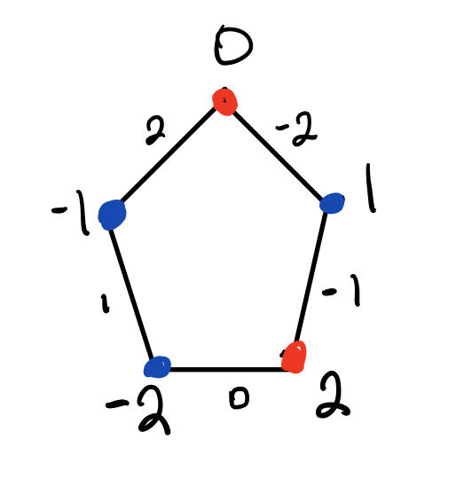
This is $C_5$, where I have labeled each vertex in $[-k,k]$, following the convention of Raz. I have also identified each edge (of which there are $m$), with its opposite vertex (also Raz's convention). The game works as follows: with probability $1/2$, the verifier will ask Alice and Bob about (the same) random vertex, and expect Alice and Bob to answer with the same color, and with probability $1/2$, the verifier will ask Alice and Bob about two neighboring vertices (so an edge), and will accept their answers if they give different labels for these two vertices. I've given a sample strategy for Alice and Bob above by choosing a coloring of the vertices, and it is not hard to see that when Alice and Bob do this, the value of the game is $1-\frac{1}{2m}$. It turns out that this is the best possible strategy.
This game turns about to be very interesting due to its relationship with foams mentioned in the first paragraph, and when this was first being explored it was shown by Feige, Kindler, and O'Donnell that $\mathsf{val}(G_{C_m}^n) \leq 1 - \frac{1}{m}\widetilde{\Omega}(\sqrt n)$, where $G_{C_m}$ is this odd-cycle game. We won't get much into this though (maybe in a later post...). What we will show today is that this is actually tight, and there is a protocol that Alice and Bob can run which achieves (for some $n \leq O(m^2)$): $$\mathsf{val}(G_{C_m}^n) \geq 1 - \frac{1}{m}O(\sqrt n).$$ Recall that $n$ is the number of parallel repetitions and $m=2k+1$ is the number of vertices in our odd-cycle. This is actually precisely the counterexample to strong parallel repetition that Raz proved! Why is it a counterexample? Well, consider $n \geq \Omega(m^2)$. Then, we can split $[n]$ into roughly $\frac{n}{\alpha m^2}$ blocks, each of size $\alpha m^2$. Then, Alice and Bob can run this protocol on each block, and we would have that $$\mathsf{val}(G_{C_m}^n) = \left(1 - \frac{1}{m}O(\sqrt{\text{block size}})\right)^{\text{# of blocks}} \approx (1-\frac{1}{4m^2})^{O(n)}.$$ The $\approx$ above just hides some computations/constants. The important thing is that this gives a protocol that achieves a value of $\Omega(1-\epsilon^2)^{O(n)}$ for the odd-cycle game, which serves as a counterexample to strong parallel repetition.
Proof Idea
I will work backwards in sketching this proof idea. Namely, let's start with some wishful thinking. Recall that Alice receives $x_1,...,x_n \in [-k,k]$ as her input and Bob receives $y_1,...,y_k \in [-k,k]$ as his input such that $y_i=x_i$ with probability $1/2$, and $y_i = \pm x_i$ with probability $1/2$. Suppose Alice and Bob could (potentially using shared randomness) agree on a set of edges $e_1,...,e_n$ of edges such that $e_i$ does not have $x_i$ as one of its endpoints for all $i \in [n]$. Then, I claim that Alice and Bob can win the repeated game with probability one. Why? Well, once they have agreed on these $n$ edges, on repetition $i$ they can simply color both vertices blue that touch $e_i$, and alternate all the other colors. We know that $x_i$ does not touch $e_i$, so the verifier will never check this edge, and Alice and Bob are guaranteed to win.
So, I have argued that all Alice and Bob need to do is agree on $e_1,...,e_n$ with this property with probability at least $1-\frac{1}{m}O(\sqrt n)$. Now, the goal is to show how to use shared randomness to actually achieve this. To do so, we need a lemma from Holenstein, which was actually used to simplify Raz's original proof of his parallel repetition theorem. Here is the lemma:
With Holenstein's lemma in hand, we are much closer. Alice and Bob's strategy will be as follows. Alice will define $P_x(e)$, which is a probability distribution on edges, defined by her input $x = (x_1,...,x_n)$, which gives the probability of her sampling a particular $e = (e_1,...,e_n)$. Bob will do the same and define $P_y(e)$. It suffices for $P_x$ and $P_y$ to have the property that 1) the statistical distance of $P_x$ and $P_y$ is on the order of $\frac{1}{m}O(\sqrt n)$ and 2) the probability that $x_i$ touches $e_i$ for any of the $e_i$ that they sample is negligible (or at least less than $\frac{1}{m}O(\sqrt n)$). By Holenstein's lemma, we would then be done! This is in fact the only technical part of Raz's proof. The distributions $P_x$ and $P_y$ are defined as product distributions over the individual rounds. Basically, suppose Alice gets $x_i$ and Bob gets $y_i \in \{x_i - 1, x_i, x_i + 1\} (\text{mod $m$})$. We just need to define a distribution that places small weight on edges that are touching/close to $x_i$ (in order to satisfy the condition that $e_i$ does not touch $x_i$), while also being smooth enough such that the statistical distance is not too much between $P_x$ and $P_y$. He achieves this by using a normalized quadratic function that has its maximum at the edge that is furthest away from the current vertex.
This is pretty much where my intuition stops (if you want to see how Raz defined $P_x$ and $P_y$, you can read through the ~1.5 pages of math in his paper that would not be so instructive for me to copy here). However, Justin Holmgren pointed me to perhaps some more intuition via this paper. Essentially, this paper explores what they call the "chi-squared" method, which is a way to bound the statistical distance of two product distributions using the chi-squared distance of the distributions of which they are made. Suppose (and this is indeed the case), that $P_x$ is a $n$-wise direct product of distributions. The "naive" way to bound the statistical distance of $P_x$ and $P_y$ would be to just multiply by $n$ the statistical distance of the individual distributions of which it is comprised. However, this paper I linked above shows that if you can bound the chi-squared distance of the individual distributions, then the statistical distance is bounded by something like $\sqrt n \delta$ (where $\delta^2$ is the chi-squared distance of the individual distributions). I think that the third condition Raz lists when defining the individual distributions of which $P_x$ and $P_y$ are comprised somehow correspond to a chi-squared distance bound. This is still a bit fuzzy to me though, and I haven't exactly formalized how this third condition corresponds to a chi-squared bound yet.
Whew. That's all for this post!